Screening Method to Estimate if a Chlorinated Solvent Release is in the Early, Late, or Middle Stage

The chlorinated solvent FAQ (Sale et al. 2008) presents the idea that chlorinated solvent sites go through various stages during their life cycle. In the early stage, chlorinated solvent releases are dominated by dense nonaqueous phase liquid (DNAPL); over time, DNAPLs slowly dissolve, plumes develop, and contaminants accumulate in permeable zones. Eventually, little to no DNAPL remains, and plumes are sustained by the release of contaminants from low-permeability zones via diffusion (Chapman and Parker 2005). Although recoverable, DNAPL can still be found within some source zones; it is very difficult to find DNAPLs at the heads of many persistent plumes. At some sites (see the “late stage” depiction in the graphic below), DNAPL may no longer be present, even though the source zone [see question 4 in Sale et al. (2008)] is still active. Key factors controlling the rate at which chlorinated solvent releases age include the amount of DNAPL released, the solubility of the constituent in the DNAPL, the rate of groundwater flow, and the architecture of transmissive and low-permeability zones.

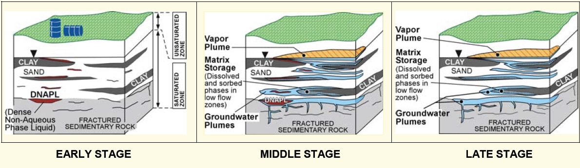
Described below is a methodology used by site managers, consultants, remediation specialists, and regulators to determine whether they are working on an early-, middle-, or late-stage site. The method is based on work experience in chlorinated solvent source zones, with some assistance from recently developed matrix diffusion models that form the basis of the Environmental Security Technology Certification Program’s Matrix Diffusion Toolkit (Farhat et al. 2012). This method is an initial classification system, and the approach may change as more is discovered about how chlorinated solvent sites age.

Figure F-1. Aging of a chlorinated solvent release.

Examples are as follows:

• My regulatory guidance says I must remove DNAPL if present (for example, DNAPL is considered a primary threat waste).
• I want to consider using a DNAPL-specific technology (such as injection-based technology).

Some key considerations about the screening method are as follows:

• It is designed for chlorinated solvent sites, although it may be possible to adapt it for other contaminants.
• Although the method can be applied to other DNAPL constituents, it is mainly derived from experience with trichoroethene (TCE) sites.
• It is relatively general and relies on several interpretations when compiling the required data; thus, different users may generate different answers.
• The method may be time intensive as it requires careful consideration about the site and the data required.

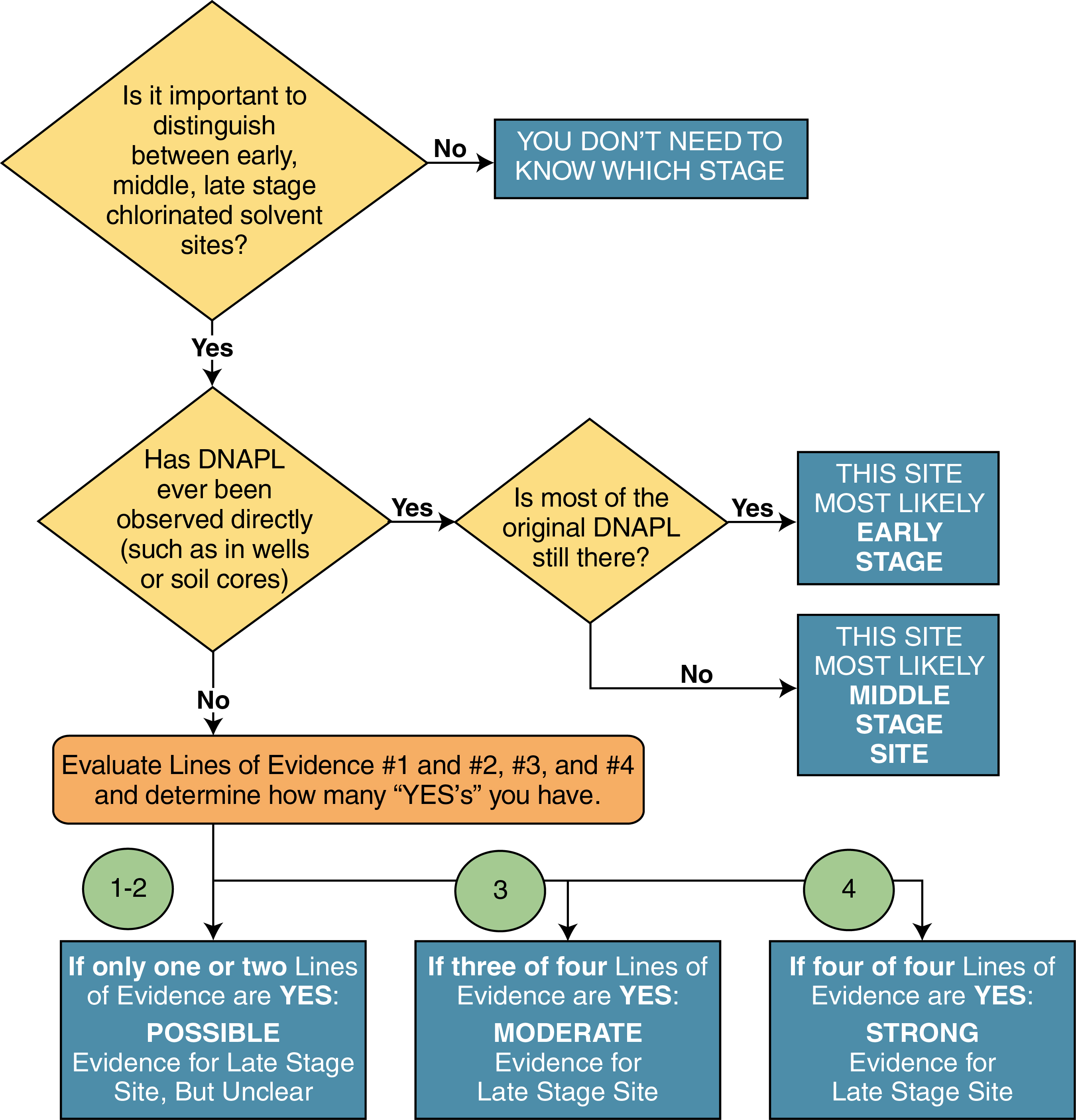
Figure F-2. Screening method decision chart.

Examples are as follows:

• I’m going to use containment.
• I'm going to use a DNAPL technology that is not DNAPL (type) specific (such as thermal remediation).

Is Most of the Original DNAPL Still There?

It can be difficult and controversial to answer questions as to whether DNAPL is still present. Some observations and speculations are presented below; these may change over time as better methods for understanding DNAPL source zones are developed. In this application, references to DNAPL mean DNAPL chemicals rather than an insoluble oil or other chemicals in the original release.

Knowing whether the original DNAPL is still present depends on several variables that can be difficult to determine, such as the amount of the release, the composition of the DNAPL, and the source architecture, as well as more commonly measured geochemical and hydrogeologic variables. Simple dissolution models can be used as guidance; however, if the DNAPL is mainly in ganglia or blob form, the resulting dissolution times are often just a few years. DNAPL pools, particularly long ones (tens of meters), can last for several decades.

In general, the answer is more likely to be "No" if the site has more of the following characteristics:

• There are only a few indicators of DNAPL presence (for example, a couple of stains on just a few cores).
• No significant DNAPL accumulation in groundwater monitoring wells has been observed.
• The source release is small (a few hundred or few thousand kilograms or less).
• The source release mechanism and the geology will spread the DNAPL into a large volume in the subsurface.
• Groundwater seepage velocities are moderate to high (tens of meters per year or more).
• An in situ remediation technology has successfully removed much of the DNAPL mass from the transmissive zone.
• The key constituents are more soluble (several hundred or thousand milligrams per liter [mg/L] or more).
• It has been several decades since most of the DNAPL was released.

In general, the answer is more likely to be "Yes" if the site has more of these characteristics:

• There are multiple indicators of DNAPL presence (for example, many cores with positive dye test results, several monitoring wells with DNAPL accumulations).
• Significant DNAPL accumulation in monitoring wells has been observed.
• The release was very large (hundreds of thousands or millions of kilograms).
• The release point and subsurface geology result in the formation of large DNAPL pools.
• Groundwater seepage velocities are low (meters per year or less).
• No remediation or DNAPL removal has occurred.
• The key constituents have relatively low solubility (tens or a few hundreds of mg/L).
• It has been just a few years since most of the DNAPL was released.

At most sites, DNAPL is never observed, so the lines of evidence outlined below must be followed.

Line of Evidence 1- Adequate DNAPL Search?

Was a thorough direct DNAPL investigation conducted, in which one or more of the following was performed:

• Interfaces above low-permeability zones were sampled.

                  OR

• A vertical transect was used to identify high flux zones that were then sampled for DNAPL.

                  OR

• Soil samples were investigated using enhanced techniques such as hydrophobic dye.

                  OR

• Other DNAPL-specific characterization technologies were used.

If ANY of these were done, Line of Evidence 1 is YES.

If NONE were done, Line of Evidence 1 is NO.

(IMPORTANT: the “1% rule” should not be used to indicate the presence of DNAPL).

Line of Evidence 2 - Old Plume + Heterogeneity?

Does the site meet both of these qualitative conditions?

• The site has low–k zones (such as silts, clays, sandstone, limestone) with hydraulic conductivity of at least 100 times lower than the fastest transmissive zones that is, or was, in contact with the plume.

                  AND

• The original release likely occurred more than 30 years ago.

If BOTH of these are TRUE, Line of Evidence 2 is YES.

If EITHER IS FALSE, Line of Evidence 2 is NO.

Line of Evidence 3 - Can the Low-k Zone Hold Enough Mass?

Calculate TCE mass per cubic meter of low-k material using Figure F-3, and estimate the volume of low-k material at the site using Figure F-4 (see figures below).

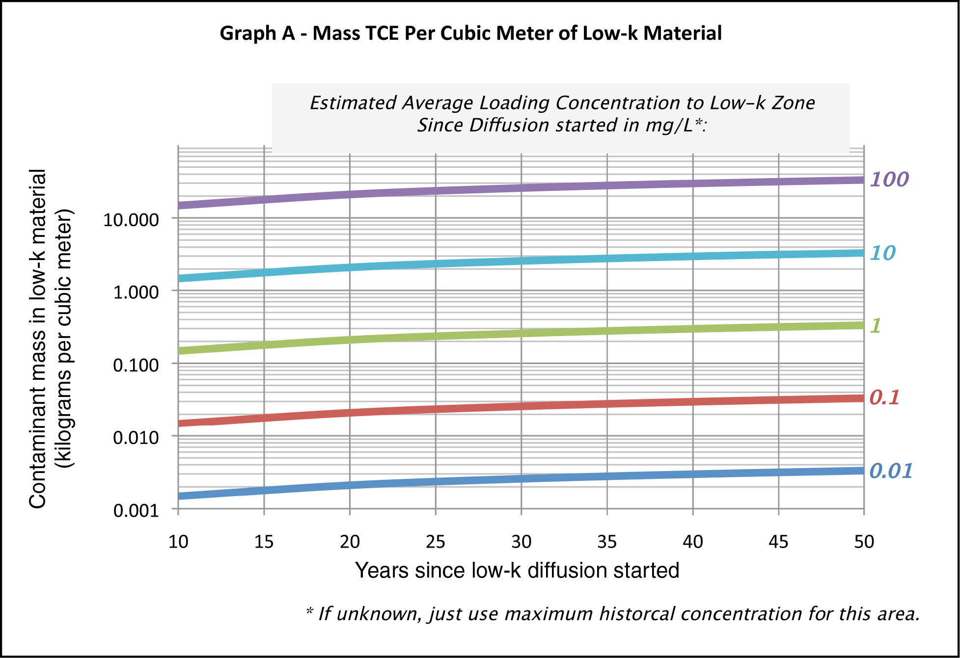
Figure F-3. Mass TCE per cubic meter of low-k material.

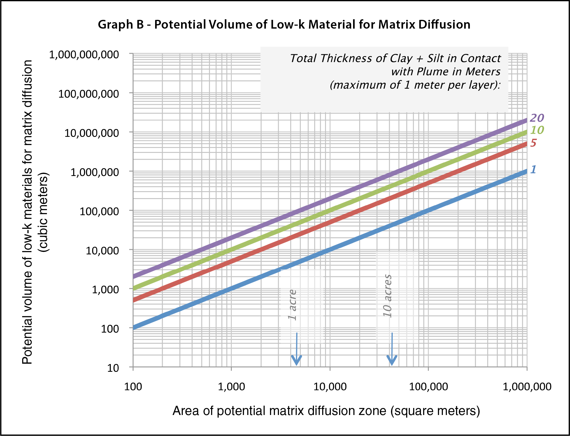
Figure F-4. Potential volume of low-k material for matrix diffusion.

Multiply the two values from Figure F-3 and Figure F-4 to get an estimated mass in low–k unit in kilograms.

This particular chart is designed for TCE and for a source zone, but can be applied to other chlorinated solvents by multiplying by the pure-phase solubility of the specific DNAPL chemical in mg/L and dividing by 1,000 mg/L (value used for TCE).

This can be done for different parts of the site – such as the original source zone; a high-concentration part of the plume and a low-concentration area, each with a different concentration; year since low-k diffusion started; and areas – and then the numbers can be added.

If the mass is >100 kg, Line of Evidence 3 is YES.

If the mass is <100 kg, Line of Evidence 3 is NO.

LINE OF EVIDENCE 4 - Can Low-k Zones Create High Enough Concentrations?

Estimate the length of the low-k zone parallel to groundwater flow that might have been in contact with a high-strength plume. Enter the graph and select the line for the subject contaminant. If the contaminant is not represented, find the line for the chemical with the solubility closest to the subject contaminant (for this graph, the solubility of 1,2-dichloroethane (DCA), cis-dichloroethene (DCE), TCE, and tetrachloroethene (PCE) were assumed to be 8,690, 1,000, 800, and 143 mg/L, respectively. Alternatively, the Matrix Diffusion Toolkit can be run to evaluate potential monitoring well concentrations from low-k zones.

At the y-axis, find the potential maximum concentration in groundwater in a monitoring well with a 10 ft screen in mg/L (note: log scale).

If the potential maximum concentration in Step 3 is greater than the maximum historical concentration for that contaminant at the site, Line of Evidence 4 is YES.

If the potential maximum concentration in Step 3 is less than the maximum historical concentration for that contaminant at the site, Line of Evidence 4 is NO.

If the mass in Step 3 is <100 kg, Line of Evidence 4 is NO.

If the calculated maximum theoretical concentration from Figure F-5 below is less than the observed maximum concentration in site monitoring wells, a late-stage site is possible and Line of Evidence 4 is YES; otherwise, Line of Evidence 4 is NO.

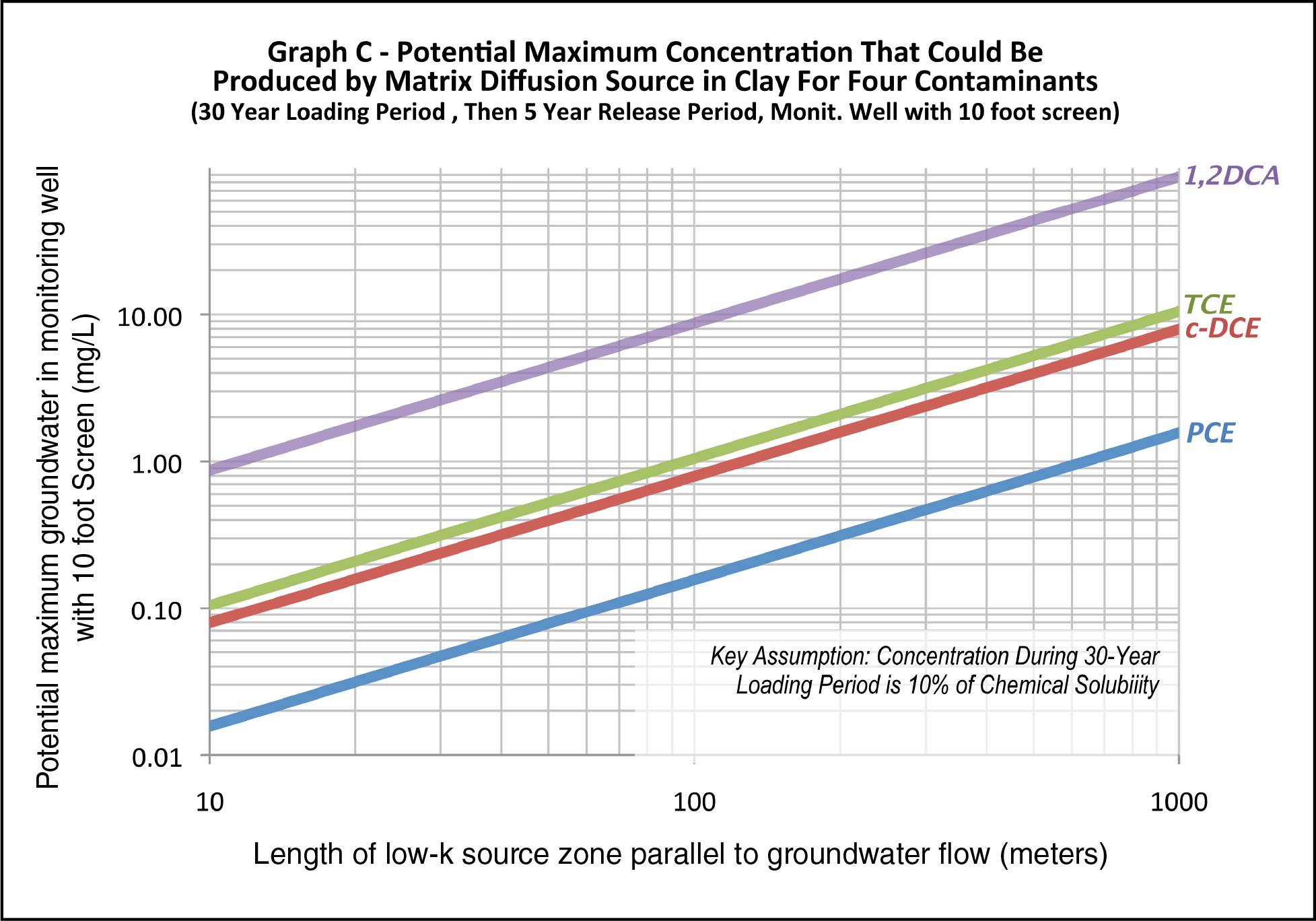
Figure F-5. Potential maximum concentration that could be produced by matrix diffusion source in clay for four contaminants (30-year loading period, then 5-year release period, monitoring well with 10 ft screen).

Technical Basis- How Does This Work?

The methodology for matrix diffusion modeling is discussed in the following sections.

Overall Basis – Assume Simple Geometry, One Low-k Unit, One Transmissive Unit

This methodology is designed for sites with unconsolidated hydrogeologic settings (sand, silt, clay), with a single low-k unit in contact with a plume in a transmissive zone. For those familiar with matrix diffusion modeling, the methodology can be adapted to other configurations such as multi-layered systems and fractured rock sites by multiplying the results in Lines of Evidence 3 and 4 (below) by the number of contacts between transmissive and low-k units.

Line of Evidence 1 – Adequate DNAPL Search?

A strong but not conclusive line of evidence of a late-stage site is that a thorough search for DNAPL using current DNAPL-specific techniques did not reveal any evidence of DNAPL in the source zone. Determining if a particular field program rates a YES or NO is somewhat subjective, but the main criterion is that a DNAPL-specific field investigation to find direct evidence of DNAPL in wells and soil cores was performed. Use of the 1% should not be used for Line of Evidence 1 because matrix diffusion modeling indicates that strong matrix diffusion sources can create concentrations greater than 1% of the effective solubility of DNAPL.

Line of Evidence 2 – Old Plume + Heterogeneity?

There are two key ingredients for a strong, long-lived matrix diffusion source: (1) heterogeneity, considering that a 100-fold difference in hydraulic conductivity leads to matrix diffusion processes (B. Parker, University of Guelph, personal communication); and (2) old sites loading more mass in low-k zones.

Line of Evidence 3 – Can the Low-k Zone Hold Enough Mass?

The square root model in the Matrix Diffusion Toolkit (Farhat et al. 2012) is used to estimate a contaminant mass that could diffuse into a single low-k layer at least 1 m thick. The total thickness of the clay and silt in contact with a plume is then applied to the calculated potential mass per cubic meter. A site can be broken up into different zones. This method can then be used to estimate the mass separately— in high-, medium-, and low-concentration zones—and then the masses are added together.

Why 100 kg? This is the amount that can sustain an average plume (Mag 5 plume in the plume magnitude system) for 50 years (Newell et al. 2011).

Line of Evidence 4 – Can Low-k Zones Create High Enough Concentrations?

This line of evidence assumes that a plume with concentrations at 10% of the pure-phase solubility of the contaminant was in contact with a low-k zone for 30 years. If unknown, assume the length of the low-k zone is the length of the source zone at the site parallel to groundwater flow. The low-k zone was assumed to be clay with a fraction organic carbon (f_oc) of 0.002 grams per gram, giving retardation factors for DCA, DCE, TCE, and PCE of 1.4, 1.7, 1.2, and 2.1 in the clay, respectively. The Matrix Diffusion Toolkit’s square root model (Farhat et al. 2012) was used to generate the concentrations as a function of the length of the low-k zone.

Different contaminants can be evaluated by picking the lines with the solubility closest to the subject contaminant. If there is process knowledge that the concentration during the loading period is different than the 10% solubility assumed above, the final result can be adjusted by the ratio of the solubility to 10% (for example, if the loading concentration was equal to 50% of TCE pure-phase solubility, multiply the concentrations on the y-axis by 5).